Example Dysmalpy 2D fitting
In this example, we use dysmalpy to measure the kinematics of galaxy GS4_43501 at \(z=1.613\). This notebook shows how to find the best fit models for the two-dimensional velocity and velocity dispersion profiles using \(\texttt{MPFIT}\) as well as \(\texttt{MCMC}\). These fits allow us to measure quantities such as the total mass (disk+bulge), the effective radius \(r_\mathrm{eff}\), dark matter fraction \(f_\mathrm{DM}\) and velocity dispersion \(\sigma_0\).
The fitting includes the following components:
Disk + Bulge
NFW halo
Constant velocity dispersion
The structure of the notebook is the following:
Setup steps
Initialize galaxy, model set, instrument
MPFIT fitting
MCMC fitting
Visualize a real MCMC example
Nested sampling fitting
Visualize a real Nested Sampling example
1) Setup steps
Import modules
from __future__ import (absolute_import, division, print_function,
                        unicode_literals)

import dysmalpy
from dysmalpy import galaxy
from dysmalpy import models
from dysmalpy import fitting
from dysmalpy import instrument
from dysmalpy import data_classes
from dysmalpy import parameters
from dysmalpy import plotting
from dysmalpy import aperture_classes
from dysmalpy import observation
from dysmalpy import config

import os
import copy

import numpy as np
import astropy.units as u
import astropy.io.fits as fits
INFO:numexpr.utils:Note: NumExpr detected 10 cores but "NUMEXPR_MAX_THREADS" not set, so enforcing safe limit of 8.
INFO:numexpr.utils:NumExpr defaulting to 8 threads.
# A check for compatibility:
import emcee
if int(emcee.__version__[0]) >= 3:
    ftype_sampler = 'h5'
else:
    ftype_sampler = 'pickle'
Setup notebook
# Setup plotting
import matplotlib as mpl
import matplotlib.pyplot as plt
%matplotlib inline

mpl.rcParams['figure.dpi']= 100
mpl.rc("savefig", dpi=300)

from IPython.core.display import Image
import logging
logger = logging.getLogger('DysmalPy')
logger.setLevel(logging.INFO)
Set data, output paths
# Data directory
dir_path = os.path.abspath(fitting.__file__)
data_dir = os.sep.join(os.path.dirname(dir_path).split(os.sep)[:-1]+["tests", "test_data", ""])
#'/YOUR/DATA/PATH/'
print(data_dir)

# Where to save output files (see examples below)
#outdir = '/Users/sedona/data/dysmalpy_test_examples/JUPYTER_OUTPUT_2D/'
outdir = '/Users/jespejo/Dropbox/Postdoc/Data/dysmalpy_test_examples/JUPYTER_OUTPUT_2D/'
/Users/jespejo/anaconda3/envs/test_dysmalpy/lib/python3.11/site-packages/dysmalpy/tests/test_data/
Load the function to tie the scale height to the disk effective radius
from dysmalpy.fitting_wrappers.tied_functions import tie_sigz_reff
Load the function to tie Mvirial to \(f_{DM}(R_e)\)
from dysmalpy.fitting_wrappers.tied_functions import tie_lmvirial_NFW
Info
Also see fitting_wrappers.tied_functions for more tied functions
2) Initialize galaxy, model set, instrument
gal = galaxy.Galaxy(z=1.613, name='GS4_43501')
mod_set = models.ModelSet()
Baryonic component: Combined Disk+Bulge
total_mass = 11.0    # M_sun
bt = 0.3             # Bulge-Total ratio
r_eff_disk = 5.0     # kpc
n_disk = 1.0
invq_disk = 5.0
r_eff_bulge = 1.0    # kpc
n_bulge = 4.0
invq_bulge = 1.0
noord_flat = True    # Switch for applying Noordermeer flattening

# Fix components
bary_fixed = {'total_mass': False,
              'r_eff_disk': False, #True,
              'n_disk': True,
              'r_eff_bulge': True,
              'n_bulge': True,
              'bt': True}

# Set bounds
bary_bounds = {'total_mass': (10, 13),
               'r_eff_disk': (1.0, 30.0),
               'n_disk': (1, 8),
               'r_eff_bulge': (1, 5),
               'n_bulge': (1, 8),
               'bt': (0, 1)}

bary = models.DiskBulge(total_mass=total_mass, bt=bt,
                        r_eff_disk=r_eff_disk, n_disk=n_disk,
                        invq_disk=invq_disk,
                        r_eff_bulge=r_eff_bulge, n_bulge=n_bulge,
                        invq_bulge=invq_bulge,
                        noord_flat=noord_flat,
                        name='disk+bulge',
                        fixed=bary_fixed, bounds=bary_bounds)

bary.r_eff_disk.prior = parameters.BoundedGaussianPrior(center=5.0, stddev=1.0)
Halo component
mvirial = 12.0
conc = 5.0
fdm = 0.5

halo_fixed = {'mvirial': False,
              'conc': True,
              'fdm':  False}
# Mvirial will be tied -- so must set 'fixed=False' for Mvirial...

halo_bounds = {'mvirial': (10, 13),
               'conc': (1, 20),
               'fdm': (0, 1)}

halo = models.NFW(mvirial=mvirial, conc=conc, fdm=fdm, z=gal.z,
                  fixed=halo_fixed, bounds=halo_bounds, name='halo')


halo.mvirial.tied = tie_lmvirial_NFW
Dispersion profile
sigma0 = 39.   # km/s
disp_fixed = {'sigma0': False}
disp_bounds = {'sigma0': (5, 300)}

disp_prof = models.DispersionConst(sigma0=sigma0, fixed=disp_fixed,
                                          bounds=disp_bounds, name='dispprof', tracer='halpha')
z-height profile
sigmaz = 0.9   # kpc
zheight_fixed = {'sigmaz': False}

zheight_prof = models.ZHeightGauss(sigmaz=sigmaz, name='zheightgaus',
                                   fixed=zheight_fixed)
zheight_prof.sigmaz.tied = tie_sigz_reff
Geometry
inc = 62.     # degrees
pa = 142.     # degrees, blue-shifted side CCW from north
xshift = 0    # pixels from center
yshift = 0    # pixels from center
vel_shift = 0 # velocity shift at center ; km/s
geom_fixed = {'inc': False,
              'pa': False,
              'xshift': False,
              'yshift': False,
              'vel_shift': False}

geom_bounds = {'inc': (52, 72),
               'pa': (132, 152),
               'xshift': (-2.5, 2.5),
               'yshift': (-2.5, 2.5),
               'vel_shift': (-100, 100)}

geom = models.Geometry(inc=inc, pa=pa, xshift=xshift, yshift=yshift, vel_shift=vel_shift,
                       fixed=geom_fixed, bounds=geom_bounds,
                       name='geom', obs_name='halpha_2D')

geom.inc.prior = parameters.BoundedSineGaussianPrior(center=62, stddev=0.1)
Add all model components to ModelSet
# Add all of the model components to the ModelSet
mod_set.add_component(bary, light=True)
mod_set.add_component(halo)
mod_set.add_component(disp_prof)
mod_set.add_component(zheight_prof)
mod_set.add_component(geom)
Set kinematic options for calculating velocity profile
mod_set.kinematic_options.adiabatic_contract = False
mod_set.kinematic_options.pressure_support = True
Set up the observation and instrument
obs = observation.Observation(name='halpha_2D', tracer='halpha')
inst = instrument.Instrument()

beamsize = 0.55*u.arcsec                 # FWHM of beam
sig_inst = 45*u.km/u.s                   # Instrumental spectral resolution

beam = instrument.GaussianBeam(major=beamsize)
lsf = instrument.LSF(sig_inst)

inst.beam = beam
inst.lsf = lsf
inst.pixscale = 0.125*u.arcsec           # arcsec/pixel
inst.fov = [27, 27]                      # (nx, ny) pixels
inst.spec_type = 'velocity'              # 'velocity' or 'wavelength'
inst.spec_step = 10*u.km/u.s             # Spectral step
inst.spec_start = -1000*u.km/u.s         # Starting value of spectrum
inst.nspec = 201                         # Number of spectral pixels

# Set the beam kernel so it doesn't have to be calculated every step
inst.set_beam_kernel()
inst.set_lsf_kernel()

# Extraction information
inst.ndim = 2                            # Dimensionality of data
inst.moment = False                      # For 1D/2D data, if True then velocities and dispersion calculated from moments
                                         # Default is False, meaning Gaussian extraction used

# Add instrument to observation
obs.instrument = inst
Load data
Load the data from file:
2D velocity, dispersion maps and error
A mask can be loaded / created as well
Put data in
Data2DclassAdd data to Galaxy object
gal_vel = fits.getdata(data_dir+'GS4_43501_Ha_vm.fits')
gal_disp = fits.getdata(data_dir+'GS4_43501_Ha_dm.fits')

err_vel = fits.getdata(data_dir+'GS4_43501_Ha_vm_err.fits')
err_disp = fits.getdata(data_dir+'GS4_43501_Ha_dm_err.fits')

mask = fits.getdata(data_dir+'GS4_43501_Ha_m.fits')

#gal_disp[(gal_disp > 1000.) | (~np.isfinite(gal_disp))] = -1e6
#mask[(gs4_disp < 0)] = 0

inst_corr = True                  # Flag for if the measured dispersion has been
                                  # corrected for instrumental resolution

# Mask NaNs:
mask[~np.isfinite(gal_vel)] = 0
gal_vel[~np.isfinite(gal_vel)] = 0.

mask[~np.isfinite(err_vel)] = 0
err_vel[~np.isfinite(err_vel)] = 0.

mask[~np.isfinite(gal_disp)] = 0
gal_disp[~np.isfinite(gal_disp)] = 0.

mask[~np.isfinite(err_disp)] = 0
err_disp[~np.isfinite(err_disp)] = 0.


# Put data in Data2D data class:
#    ** specifies data pixscale as well **
data2d = data_classes.Data2D(pixscale=inst.pixscale.value, velocity=gal_vel,
                                  vel_disp=gal_disp, vel_err=err_vel,
                                  vel_disp_err=err_disp, mask=mask,
                                  inst_corr=inst_corr)

# Use moment for extraction for example:
#     Not how data was extracted, but it's a speedup for this example.
#
#     The best practic option, if the 2D maps are extracted with gaussians,
#     is to compile the C++ extensions and pass the option 'gauss_extract_with_c=True'
#     when running fitting.fit_mpfit()
data2d.moment = True

# Add data to Observation:
obs.data = copy.deepcopy(data2d)
Define model, fit options:
obs.mod_options.oversample = 1
# Factor by which to oversample model (eg, subpixels)
# For increased precision, oversample=3 is suggested.

obs.fit_options.fit = True             # Include this observation in the fit (T/F)
obs.fit_options.fit_velocity = True    # 1D/2D: Fit velocity of observation (T/F)
obs.fit_options.fit_dispersion = True  # 1D/2D: Fit dispersion of observation (T/F)
obs.fit_options.fit_flux = False       # 1D/2D: Fit flux of observation (T/F)
Add the model set, observation to the Galaxy
gal.model = mod_set
gal.add_observation(obs)
3) MPFIT Fitting
Set up MPFITFitter fitter with fitting parameters
# Options passed to MPFIT:
maxiter = 200

fitter = fitting.MPFITFitter(maxiter=maxiter)
Set up fit/plot output options
# Output directory
outdir_mpfit = outdir+'MPFIT/'

# Output options:
do_plotting = True
plot_type = 'png'
overwrite = True

output_options = config.OutputOptions(outdir=outdir_mpfit,
                                      do_plotting=do_plotting,
                                      plot_type=plot_type,
                                      overwrite=overwrite)
Run Dysmalpy fitting: MPFIT
mpfit_results = fitter.fit(gal, output_options)
INFO:DysmalPy:*************************************
INFO:DysmalPy: Fitting: GS4_43501 using MPFIT
INFO:DysmalPy:    obs: halpha_2D
INFO:DysmalPy:        nSubpixels: 1
INFO:DysmalPy:    mvirial_tied: <function tie_lmvirial_NFW at 0x176a55da0>
INFO:DysmalPy:
MPFIT Fitting:
Start: 2024-05-02 10:47:55.313966

INFO:DysmalPy:Iter 1  CHI-SQUARE = 27260.87785  DOF = 403
   disk+bulge:total_mass = 11
   disk+bulge:r_eff_disk = 5
   halo:fdm = 0.5
   dispprof:sigma0 = 39
   geom:inc = 62
   geom:pa = 142
   geom:xshift = 0
   geom:yshift = 0
   geom:vel_shift = 0

INFO:DysmalPy:Iter 2  CHI-SQUARE = 7174.918633  DOF = 403
   disk+bulge:total_mass = 11.01621875
   disk+bulge:r_eff_disk = 5.697081099
   halo:fdm = 0.290454085
   dispprof:sigma0 = 41.78914475
   geom:inc = 72
   geom:pa = 142.4487865
   geom:xshift = 0.01555573571
   geom:yshift = -0.01483259239
   geom:vel_shift = 0.688311908

INFO:DysmalPy:Iter 3  CHI-SQUARE = 4845.547462  DOF = 403
   disk+bulge:total_mass = 11.00485748
   disk+bulge:r_eff_disk = 7.299527889
   halo:fdm = 0.3316062539
   dispprof:sigma0 = 35.80898768
   geom:inc = 72
   geom:pa = 142.6165451
   geom:xshift = 0.00498880543
   geom:yshift = -0.01907966512
   geom:vel_shift = 1.26046722

INFO:DysmalPy:Iter 4  CHI-SQUARE = 4135.278964  DOF = 403
   disk+bulge:total_mass = 10.97290392
   disk+bulge:r_eff_disk = 5.906465959
   halo:fdm = 0.2268716489
   dispprof:sigma0 = 39.19735991
   geom:inc = 72
   geom:pa = 142.9235737
   geom:xshift = 0.006769462096
   geom:yshift = -0.04087333416
   geom:vel_shift = 3.910223933

INFO:DysmalPy:Iter 5  CHI-SQUARE = 2681.1139  DOF = 403
   disk+bulge:total_mass = 10.99187836
   disk+bulge:r_eff_disk = 5.260076359
   halo:fdm = 0.06304476313
   dispprof:sigma0 = 35.0014785
   geom:inc = 72
   geom:pa = 144.7019383
   geom:xshift = 0.005638298412
   geom:yshift = -0.08458184636
   geom:vel_shift = 13.29443606

INFO:DysmalPy:Iter 6  CHI-SQUARE = 1975.039779  DOF = 403
   disk+bulge:total_mass = 11.01752643
   disk+bulge:r_eff_disk = 5.972062778
   halo:fdm = 0.07041719829
   dispprof:sigma0 = 33.79762307
   geom:inc = 72
   geom:pa = 144.82705
   geom:xshift = 0.003838933716
   geom:yshift = -0.08965685046
   geom:vel_shift = 22.53154176

INFO:DysmalPy:Iter 7  CHI-SQUARE = 1911.611202  DOF = 403
   disk+bulge:total_mass = 11.02762255
   disk+bulge:r_eff_disk = 6.236754678
   halo:fdm = 0.07706825794
   dispprof:sigma0 = 35.78878353
   geom:inc = 72
   geom:pa = 145.0908239
   geom:xshift = 0.002765540566
   geom:yshift = -0.08522907649
   geom:vel_shift = 24.69604616

INFO:DysmalPy:Iter 8  CHI-SQUARE = 1874.721763  DOF = 403
   disk+bulge:total_mass = 11.05717868
   disk+bulge:r_eff_disk = 6.756909482
   halo:fdm = 0.08265623498
   dispprof:sigma0 = 36.07195236
   geom:inc = 72
   geom:pa = 145.1249566
   geom:xshift = 0.002925563871
   geom:yshift = -0.09434522976
   geom:vel_shift = 24.74136223

INFO:DysmalPy:Iter 9  CHI-SQUARE = 1868.205783  DOF = 403
   disk+bulge:total_mass = 11.07330048
   disk+bulge:r_eff_disk = 6.976880571
   halo:fdm = 0.08303211692
   dispprof:sigma0 = 39.11660957
   geom:inc = 72
   geom:pa = 145.0231882
   geom:xshift = 0.002306094135
   geom:yshift = -0.1027435952
   geom:vel_shift = 24.51481928

INFO:DysmalPy:Iter 10  CHI-SQUARE = 1834.891502  DOF = 403
   disk+bulge:total_mass = 11.12364485
   disk+bulge:r_eff_disk = 7.783313281
   halo:fdm = 0.05379420088
   dispprof:sigma0 = 35.87322102
   geom:inc = 72
   geom:pa = 145.0823943
   geom:xshift = 0.002328402216
   geom:yshift = -0.1072879964
   geom:vel_shift = 24.3734785

INFO:DysmalPy:Iter 11  CHI-SQUARE = 1804.57498  DOF = 403
   disk+bulge:total_mass = 11.15233343
   disk+bulge:r_eff_disk = 8.49550137
   halo:fdm = 0.05314505098
   dispprof:sigma0 = 35.22862485
   geom:inc = 72
   geom:pa = 145.2209654
   geom:xshift = 0.00213117077
   geom:yshift = -0.1118302835
   geom:vel_shift = 25.7821227

INFO:DysmalPy:Iter 12  CHI-SQUARE = 1765.875956  DOF = 403
   disk+bulge:total_mass = 11.1995498
   disk+bulge:r_eff_disk = 9.671163543
   halo:fdm = 0.0567955085
   dispprof:sigma0 = 33.6639676
   geom:inc = 72
   geom:pa = 145.1054693
   geom:xshift = 0.001771156208
   geom:yshift = -0.1214819783
   geom:vel_shift = 25.15294892

INFO:DysmalPy:Iter 13  CHI-SQUARE = 1750.678931  DOF = 403
   disk+bulge:total_mass = 11.23072663
   disk+bulge:r_eff_disk = 10.71370417
   halo:fdm = 0.06951073943
   dispprof:sigma0 = 33.20391113
   geom:inc = 72
   geom:pa = 145.5238662
   geom:xshift = 0.001667999645
   geom:yshift = -0.1229693221
   geom:vel_shift = 25.23407271

INFO:DysmalPy:Iter 14  CHI-SQUARE = 1749.269119  DOF = 403
   disk+bulge:total_mass = 11.20953224
   disk+bulge:r_eff_disk = 10.26453885
   halo:fdm = 0.07783456653
   dispprof:sigma0 = 33.20999322
   geom:inc = 72
   geom:pa = 145.2975363
   geom:xshift = 0.00150466758
   geom:yshift = -0.1259508646
   geom:vel_shift = 25.64745219

INFO:DysmalPy:Iter 15  CHI-SQUARE = 1742.263826  DOF = 403
   disk+bulge:total_mass = 11.26350202
   disk+bulge:r_eff_disk = 11.69794866
   halo:fdm = 0.06604308184
   dispprof:sigma0 = 30.21624009
   geom:inc = 72
   geom:pa = 145.2839822
   geom:xshift = 0.001305084891
   geom:yshift = -0.1274298711
   geom:vel_shift = 24.36968127

INFO:DysmalPy:Iter 16  CHI-SQUARE = 1739.337454  DOF = 403
   disk+bulge:total_mass = 11.27240108
   disk+bulge:r_eff_disk = 12.14000166
   halo:fdm = 0.06225635304
   dispprof:sigma0 = 29.57297226
   geom:inc = 72
   geom:pa = 145.3862099
   geom:xshift = 0.001253914203
   geom:yshift = -0.1281740116
   geom:vel_shift = 25.17378889

INFO:DysmalPy:Iter 17  CHI-SQUARE = 1739.259112  DOF = 403
   disk+bulge:total_mass = 11.27160988
   disk+bulge:r_eff_disk = 12.16727606
   halo:fdm = 0.06791349056
   dispprof:sigma0 = 29.6275998
   geom:inc = 72
   geom:pa = 145.5798563
   geom:xshift = 0.00125420715
   geom:yshift = -0.1281740091
   geom:vel_shift = 25.16057188

INFO:DysmalPy:Iter 18  CHI-SQUARE = 1739.231006  DOF = 403
   disk+bulge:total_mass = 11.27124049
   disk+bulge:r_eff_disk = 12.16817228
   halo:fdm = 0.06921169832
   dispprof:sigma0 = 29.36534085
   geom:inc = 72
   geom:pa = 145.5474635
   geom:xshift = 0.0012542433
   geom:yshift = -0.1281740091
   geom:vel_shift = 25.16393383

INFO:DysmalPy:Iter 19  CHI-SQUARE = 1739.16602  DOF = 403
   disk+bulge:total_mass = 11.27116728
   disk+bulge:r_eff_disk = 12.16748897
   halo:fdm = 0.06849834081
   dispprof:sigma0 = 29.39382619
   geom:inc = 72
   geom:pa = 145.5310079
   geom:xshift = 0.001254262134
   geom:yshift = -0.1281740093
   geom:vel_shift = 25.16345192

INFO:DysmalPy:Iter 20  CHI-SQUARE = 1739.088768  DOF = 403
   disk+bulge:total_mass = 11.27103747
   disk+bulge:r_eff_disk = 12.16351352
   halo:fdm = 0.06834328557
   dispprof:sigma0 = 29.48910938
   geom:inc = 72
   geom:pa = 145.5112834
   geom:xshift = 0.001254247263
   geom:yshift = -0.12817401
   geom:vel_shift = 25.16981092

INFO:DysmalPy:Iter 21  CHI-SQUARE = 1739.068692  DOF = 403
   disk+bulge:total_mass = 11.27103113
   disk+bulge:r_eff_disk = 12.1637523
   halo:fdm = 0.06841855337
   dispprof:sigma0 = 29.56525146
   geom:inc = 72
   geom:pa = 145.5131879
   geom:xshift = 0.001254248468
   geom:yshift = -0.12817401
   geom:vel_shift = 25.17058334

INFO:DysmalPy:Iter 22  CHI-SQUARE = 1739.068121  DOF = 403
   disk+bulge:total_mass = 11.27101952
   disk+bulge:r_eff_disk = 12.16317579
   halo:fdm = 0.06840690692
   dispprof:sigma0 = 29.52972761
   geom:inc = 72
   geom:pa = 145.5064353
   geom:xshift = 0.001254248505
   geom:yshift = -0.12817401
   geom:vel_shift = 25.17074722

INFO:DysmalPy:
End: 2024-05-02 10:48:07.465394

******************
Time= 12.15 (sec),   0:12.15 (m:s)
MPFIT Status = 2
MPFIT Error/Warning Message = None
******************
Examine MPFIT results
Result plots
# Look at best-fit:
filepath = outdir_mpfit+"GS4_43501_mpfit_bestfit_halpha_2D.{}".format(plot_type)
Image(filename=filepath, width=600)

Directly generating result plots
Reload the galaxy, results files:
f_galmodel =       outdir_mpfit + 'GS4_43501_model.pickle'
f_mpfit_results =  outdir_mpfit + 'GS4_43501_mpfit_results.pickle'

gal, mpfit_results = fitting.reload_all_fitting(filename_galmodel=f_galmodel,
                            filename_results=f_mpfit_results, fit_method='mpfit')
Plot the best-fit results:
mpfit_results.plot_results(gal)

Result reports
We now look at the results reports, which include the best-fit values and uncertainties (as well as other fitting settings and output).
# Print report
print(mpfit_results.results_report(gal=gal))
###############################
 Fitting for GS4_43501

Date: 2024-05-02 10:48:08.695418

    obs: halpha_2D
         Datafiles:
         fit_velocity:           True
         fit_dispersion:         True
         fit_flux:               False
         moment:           False
         n_wholepix_z_min:      3
         oversample:            1
         oversize:              1


Fitting method: MPFIT
    fit status: 2

pressure_support:      True
pressure_support_type: 1

###############################
 Fitting results
-----------
 disk+bulge
    total_mass         11.2710  +/-   0.0105
    r_eff_disk         12.1632  +/-   0.3596

    n_disk              1.0000  [FIXED]
    r_eff_bulge         1.0000  [FIXED]
    n_bulge             4.0000  [FIXED]
    bt                  0.3000  [FIXED]
    mass_to_light       1.0000  [FIXED]

    noord_flat          True
-----------
 halo
    fdm                 0.0684  +/-   0.0017

    mvirial            10.3144  [TIED]
    conc                5.0000  [FIXED]
-----------
 dispprof
    sigma0             29.5297  +/-   1.0188
-----------
 zheightgaus
    sigmaz              2.0661  [TIED]
-----------
 geom
    inc                72.0000  +/-   0.0000
    pa                145.5064  +/-   0.3302
    xshift              0.0013  +/-   0.0001
    yshift             -0.1282  +/-   0.0056
    vel_shift          25.1707  +/-   0.4656

-----------
Adiabatic contraction: False

-----------
Red. chisq: 4.3153

-----------
obs halpha_2D: Rout,max,2D: 10.3258
To directly save the results report to a file, we can use the following:
(Note: by default, report files are saved as part of the fitting process)
# Save report to file:
f_mpfit_report = outdir_mpfit + 'mpfit_fit_report.txt'
mpfit_results.results_report(gal=gal, filename=f_mpfit_report)
4) MCMC Fitting
Get a clean copy of model, obs
gal = galaxy.Galaxy(z=1.613, name='GS4_43501')

obscopy = observation.Observation(name='halpha_2D', tracer='halpha')
obscopy.data = copy.deepcopy(data2d)
obscopy.instrument = copy.deepcopy(inst)
obscopy.mod_options = copy.deepcopy(obs.mod_options)
obscopy.fit_options = copy.deepcopy(obs.fit_options)

gal.add_observation(obscopy)

gal.model = copy.deepcopy(mod_set)
Set up MCMCFitter fitter with fitting parameters
# Options passed to emcee
## SHORT TEST:
nWalkers = 20
nCPUs = 4
scale_param_a = 5 #3
# The walkers were not exploring the parameter space well with scale_param_a = 3,
#     but were getting 'stuck'. So to improve the walker movement with larger
#     'stretch' in the steps, we increased scale_param_a.
nBurn = 2
nSteps = 5
minAF = None
maxAF = None
nEff = 10

blob_name = 'mvirial'    # Also save 'blob' values of Mvirial, calculated at every chain step


fitter = fitting.MCMCFitter(nWalkers=nWalkers, nCPUs=nCPUs,
                            scale_param_a=scale_param_a, nBurn=nBurn, nSteps=nSteps,
                            minAF=minAF, maxAF=maxAF, nEff=nEff, blob_name=blob_name)
Set up fit/plot output options
# Output directory
outdir_mcmc = outdir + 'MCMC/'

# Output options:
do_plotting = True
plot_type = 'png'
overwrite = True

output_options = config.OutputOptions(outdir=outdir_mcmc,
                                      do_plotting=do_plotting,
                                      plot_type=plot_type,
                                      overwrite=overwrite)
Run Dysmalpy fitting: MCMC
mcmc_results = fitter.fit(gal, output_options)
INFO:DysmalPy:*************************************
INFO:DysmalPy: Fitting: GS4_43501 with MCMC
INFO:DysmalPy:    obs: halpha_2D
INFO:DysmalPy:        nSubpixels: 1
INFO:DysmalPy:
nCPUs: 4
INFO:DysmalPy:nWalkers: 20
INFO:DysmalPy:lnlike: oversampled_chisq=True
INFO:DysmalPy:
blobs: mvirial
INFO:DysmalPy:
mvirial_tied: <function tie_lmvirial_NFW at 0x176a55da0>
INFO:DysmalPy:
Burn-in:
Start: 2024-05-02 10:48:08.778789

INFO:DysmalPy: k=0, time.time=2024-05-02 10:48:08.779474, a_frac=nan
INFO:DysmalPy: k=1, time.time=2024-05-02 10:48:09.729780, a_frac=0.25
INFO:DysmalPy:
End: 2024-05-02 10:48:10.247523

******************
nCPU, nParam, nWalker, nBurn = 4, 9, 20, 2
Scale param a= 5
Time= 1.47 (sec),   0:1.47 (m:s)
Mean acceptance fraction: 0.225
Ideal acceptance frac: 0.2 - 0.5
Autocorr est: [nan nan nan nan nan nan nan nan nan]
******************
INFO:DysmalPy:
Ensemble sampling:
Start: 2024-05-02 10:48:10.973361

INFO:DysmalPy:ii=0, a_frac=0.2 time.time()=2024-05-02 10:48:11.308325
INFO:DysmalPy:0: acor_time =[nan nan nan nan nan nan nan nan nan]
INFO:DysmalPy:ii=1, a_frac=0.175 time.time()=2024-05-02 10:48:11.514939
INFO:DysmalPy:1: acor_time =[nan nan nan nan nan nan nan nan nan]
INFO:DysmalPy:ii=2, a_frac=0.18333333333333335 time.time()=2024-05-02 10:48:12.045867
INFO:DysmalPy:2: acor_time =[nan nan nan nan nan nan nan nan nan]
INFO:DysmalPy:ii=3, a_frac=0.2125 time.time()=2024-05-02 10:48:12.293471
INFO:DysmalPy:3: acor_time =[nan nan nan nan nan nan nan nan nan]
INFO:DysmalPy:ii=4, a_frac=0.22000000000000006 time.time()=2024-05-02 10:48:12.597950
INFO:DysmalPy:4: acor_time =[nan nan nan nan nan nan nan nan nan]
INFO:DysmalPy:Finished 5 steps

INFO:DysmalPy:
End: 2024-05-02 10:48:12.608378

******************
nCPU, nParam, nWalker, nSteps = 4, 9, 20, 5
Scale param a= 5
Time= 1.63 (sec),   0:1.63 (m:s)
Mean acceptance fraction: 0.220
Ideal acceptance frac: 0.2 - 0.5
Autocorr est: [nan nan nan nan nan nan nan nan nan]
******************
WARNING:root:Too few points to create valid contours
WARNING:root:Too few points to create valid contours
WARNING:root:Too few points to create valid contours
WARNING:root:Too few points to create valid contours
Examine MCMC results
Of course this (very short!) example looks terrible, but it’s instructive to see what’s happening even if you only did a very short / few walker MCMC test:
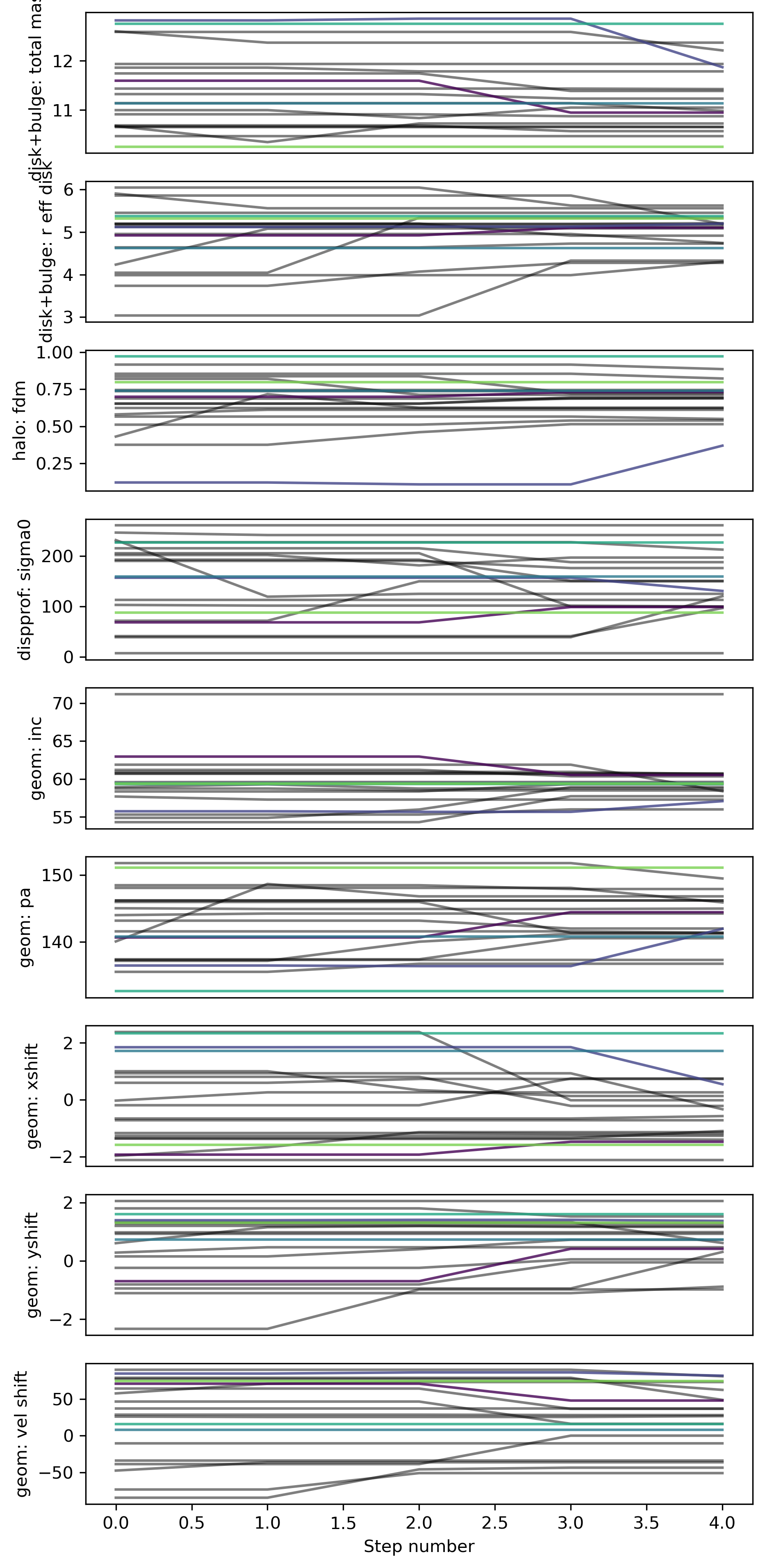
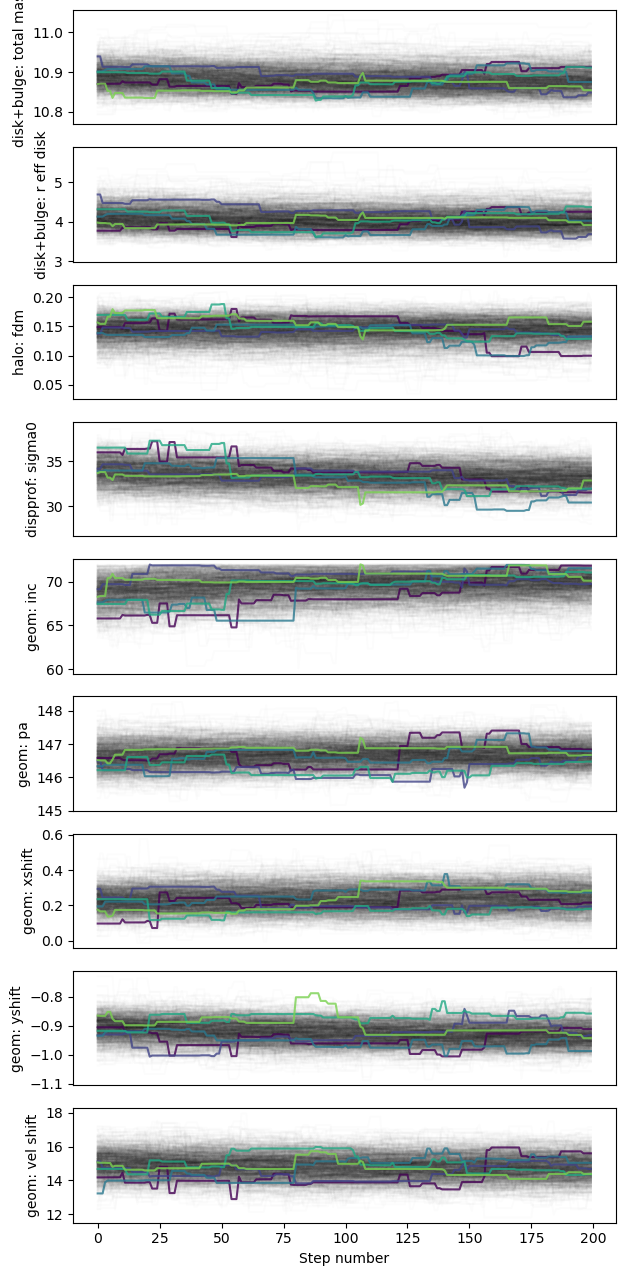
Trace
The individual walkers should move around in the parameter space over the chain iterations (not necessarily for every step; but there should be some exploration of the space)
# Look at trace:
filepath = outdir_mcmc+"GS4_43501_mcmc_trace.{}".format(plot_type)
Image(filepath, width=600)
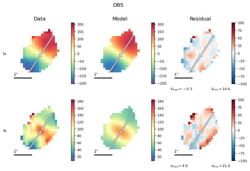
Best-fit
This is a good opportunity to check that the model PA and slit PA are correct, or else the data and model curves will have opposite shapes!
Also, it’s helpful to check that your data masking is reasonable.
Finally, this is a worthwhile chance to see if your “nuisance” geometry and spectral parameters (especially
xshift,yshift,vel_shifthave reasonable values, and if appropriate, reasonable bounds and priors.)
# Look at best-fit:
filepath = outdir_mcmc+"GS4_43501_mcmc_bestfit_halpha_2D.{}".format(plot_type)
Image(filepath, width=600)

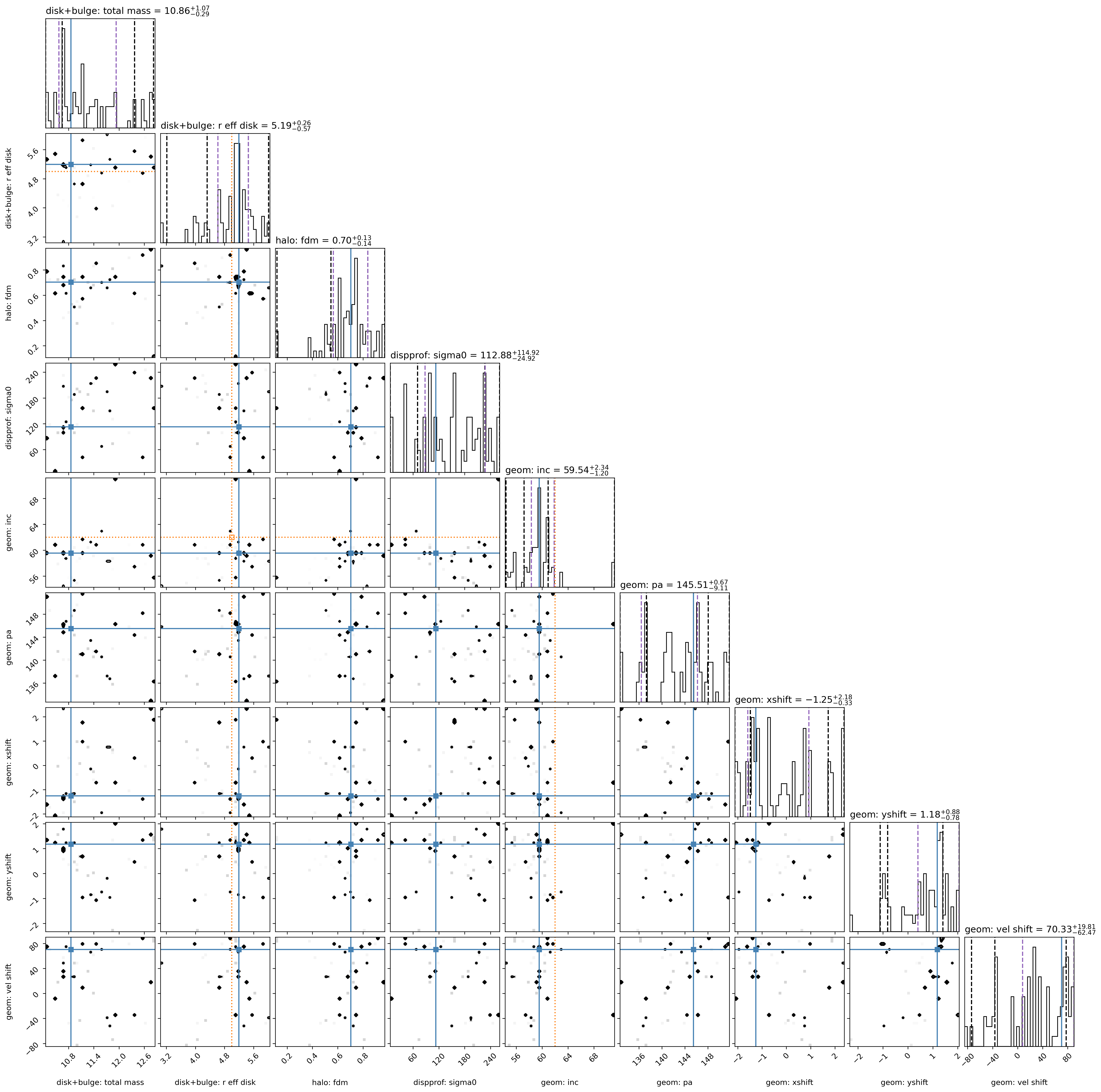
Sampler “corner” plot
The “best-fit” MAP (by default taken to be the peak of each marginalized parameter posterior, independent of the other parameters) is marked with the solid blue line.
However, the MAP can also be found by jointly analyzing two or more parameters’ posterior space.
(→ see the example in the :ref:
1D example fit <dysmalpy_example_fit_1D.ipynb>tutorial)
Check to see that your Gaussian prior centers are marked in orange in the appropriate rows/columns (if any Gaussian priors are used).
The vertical dashed black lines show the 2.275%, 15.865%, 84.135%, 97.725% percentile intervals for the marginalized posterior for each parameter.
The vertical dashed purple lines show the shortest \(1\sigma\) interval, determined from the marginalized posterior for each parameter independently.
# Look at corner:
filepath = outdir_mcmc+"GS4_43501_mcmc_param_corner.{}".format(plot_type)
Image(filepath, height=620)
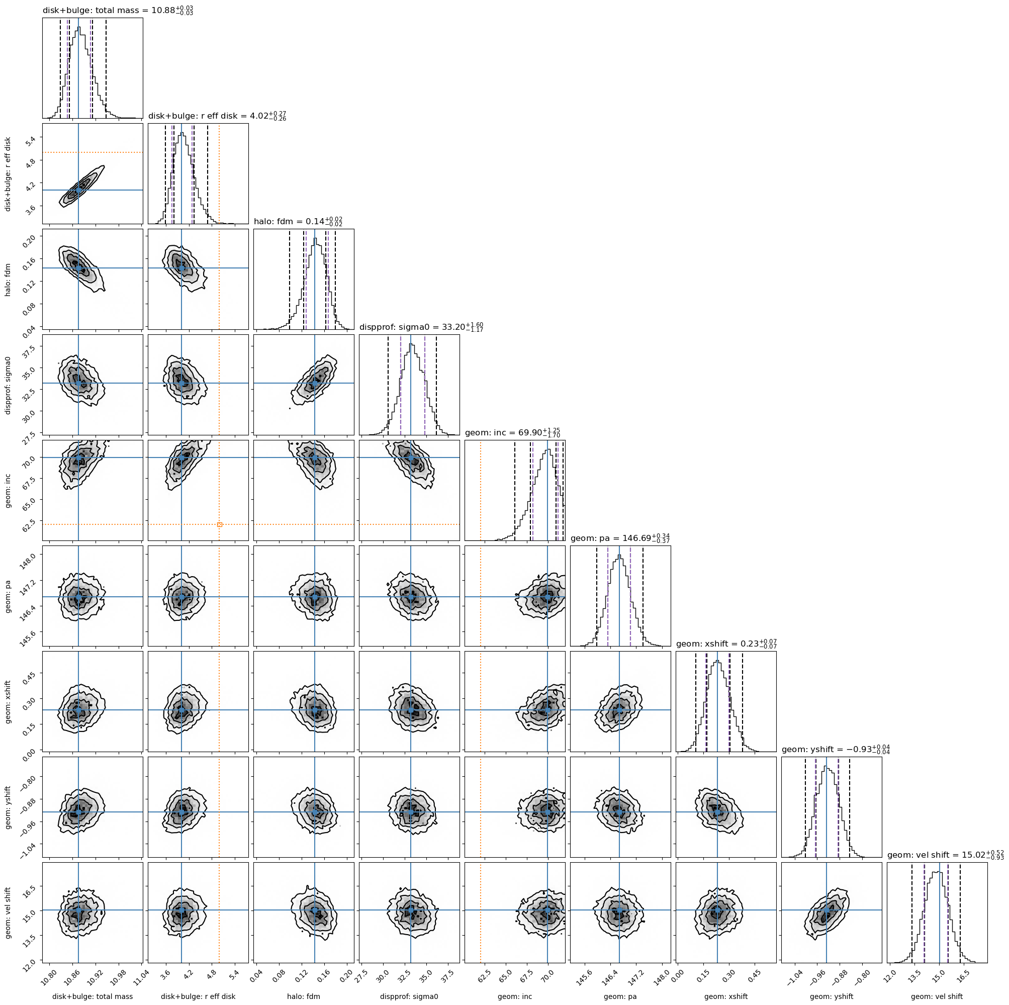
5) Visualize a real MCMC example
In the interest of time, let’s look at some results calculated previously, using 1000 walkers, 175 burn-in steps, and 200 steps.
Using 190 threads, it took about 21 minutes to run the MCMC fit.
First, you need to download the sampler from:
https://www.mpe.mpg.de/resources/IR/DYSMALPY/dysmalpy_optional_extra_files/JUPYTER_OUTPUT_2D.tar.gz
Decompress it in your preferred path (e.g.: /path/to/your/directory) and then set an environment variable to access that directory from this notebook. You can do that from the terminal running:
export DATADIR=/path/to/your/directory
Or, you can simply run the bash command from within the notebook as:
%env FULL_MCMC_RUNS_DATADIR=/path/to/your/directory
# A working example using the path of one of the maintainers:
%env FULL_MCMC_RUNS_DATADIR=/Users/jespejo/Dropbox/dysmalpy_example_files/JUPYTER_OUTPUT_2D/
env: FULL_MCMC_RUNS_DATADIR=/Users/jespejo/Dropbox/dysmalpy_example_files/JUPYTER_OUTPUT_2D/
# Now, add the environment variable to retrieve the data
_full_mcmc_runs = os.getenv('FULL_MCMC_RUNS_DATADIR')
Note
We used moment extraction for the model 2D profile extraction, as this does not seem to change the result much compared to gaussian extraction (as the observed maps were derived). This is likely because the extraction is over single pixels, so there is less complex line shape mixing as found in 1D extractions.
If this fit is done using a gaussian extraction, exactly following the data extraction method, it is generally slower.
When performing fits using moment extraction on data that was gaussian extracted, it is worth considering whether this is a reasonable thing to be doing. (Or at least check the final results with a gaussian extraction to see if there are systematic differences between the moment and gaussian maps.)
outdir_mcmc_full = _full_mcmc_runs + '/MCMC_full_run_nw1000_ns200_a5/'
Examine results:
Helpful for:
replotting
reanalyzing chain (eg, jointly constraining some posteriors)
Reload the galaxy, results files:
f_galmodel = outdir_mcmc_full + 'galaxy_model.pickle'
f_mcmc_results =  outdir_mcmc_full + 'mcmc_results.pickle'

#----------------------------------------
## Fix module import
import sys
from dysmalpy import fitting_wrappers
sys.modules['fitting_wrappers'] = fitting_wrappers
#----------------------------------------


if os.path.isfile(f_galmodel) & os.path.isfile(f_mcmc_results):
    gal_full, mcmc_results = fitting.reload_all_fitting(filename_galmodel=f_galmodel,
                                filename_results=f_mcmc_results, fit_method='mcmc')
else:
    gal_full = mcmc_results = None
If necessary, also reload the sampler chain:
f_sampler =  outdir_mcmc_full + 'mcmc_sampler.{}'.format(ftype_sampler)
if os.path.isfile(f_sampler) & (mcmc_results is not None):
    mcmc_results.reload_sampler_results(filename=f_sampler)
WARNING:emcee.autocorr:The chain is shorter than 10 times the integrated autocorrelation time for 1 parameter(s). Use this estimate with caution and run a longer chain!
N/10 = 20;
tau: [19.6537326  19.9891195  19.55235249 19.98314067 19.7486466  19.41789169
 19.19654616 20.31377879 19.68237055]
Plot the best-fit results:
if (gal_full is not None) & (mcmc_results is not None):
    mcmc_results.plot_results(gal_full)
Results report:
# Print report
if (gal_full is not None) & (mcmc_results is not None):
    print(mcmc_results.results_report(gal=gal_full))
###############################
 Fitting for GS4_43501

Date: 2024-05-02 10:48:21.959682

    obs: OBS
         Datafiles:
         fit_velocity:           True
         fit_dispersion:         True
         fit_flux:               False
         moment:           True
         n_wholepix_z_min:      3
         oversample:            1
         oversize:              1


Fitting method: MCMC

pressure_support:      True
pressure_support_type: 1

###############################
 Fitting results
-----------
 disk+bulge
    total_mass         10.8755  -   0.0278 +   0.0312
    r_eff_disk          4.0151  -   0.2608 +   0.2707

    n_disk              1.0000  [FIXED]
    r_eff_bulge         1.0000  [FIXED]
    n_bulge             4.0000  [FIXED]
    bt                  0.3000  [FIXED]

    noord_flat          True
-----------
 halo
    fdm                 0.1433  -   0.0150 +   0.0242

    mvirial            11.4323  [TIED]
    conc                5.0000  [FIXED]
-----------
 dispprof
    sigma0             33.2030  -   1.1670 +   1.6011
-----------
 zheightgaus
    sigmaz              0.6820  [TIED]
-----------
 geom
    inc                69.8972  -   1.6953 +   1.2540
    pa                146.6866  -   0.3726 +   0.3369
    xshift              0.2318  -   0.0688 +   0.0688
    yshift             -0.9261  -   0.0410 +   0.0396
    vel_shift          15.0223  -   0.9314 +   0.5174

-----------
    mvirial            11.4323  -   0.1467 +   0.1957

-----------
Adiabatic contraction: False

-----------
Red. chisq: 2.3761

-----------
obs OBS: Rout,max,2D: 10.8553
Or save results report to file:
# Save report to file:
f_mcmc_report = outdir_mcmc + 'mcmc_fit_report.txt'
if (gal_full is not None) & (mcmc_results is not None):
    mcmc_results.results_report(gal=gal_full, filename=f_mcmc_report)